Transfer Learning for Industrial Visual Inspection

What is Transfer Learning?

In 2012, Alex Krizhevsky introduced AlexNet1¹, a convolutional neural network (CNN) that overwhelmingly outperformed existing vision algorithms on the ImageNet dataset. Ever since then, CNN has been extensively applied in vision inspection. However, a fatal flaw of CNN compared to existing vision algorithms is that it requires a large amount of data. Because of this problem, early CNN has been mainly applied to datasets consisting of many images, such as ImageNet.

Many researchers have pondered how to apply CNN to domains with less data, and one result is “transfer learning”. Transfer learning is a learning methodology that transfers knowledge learned in a domain with a lot of data (source domain) to a domain with little data (target domain). In CNN, transfer learning mainly involves initializing the weight values for training the target domain with the weight values learned from the source domain.

Reflection on the Similarity Between the Source Domain and Target Domain Used in Transfer Learning Research

Since 2014, transfer learning has been widely applied in CNN research. However, in most of such research, the source domain and target domain were set as datasets with the same characteristics. Yet, the industry that SAIGE is focusing on is manufacturing. Using the DAGM dataset2², we compared how different the images in the manufacturing domain are from the images in ImageNet, which is mainly used in academia.

DAGM is a dataset that creates virtual defects on fiber-shaped backgrounds, and the image appearance is very different from the ImageNet dataset, as shown in [Figure 1]. [Figure 2] shows the result of passing the source domain and target domain images through the same CNN to extract the feature vector and then projecting them in a two-dimensional space with PCA and t-SNE. The CNN also recognizes that the characteristics of these two datasets are different.

Therefore, to effectively apply transfer learning as in previous studies, it seems necessary to have a source domain dataset with similar characteristics to the manufacturing domain data we are targeting. However, since the product data held by each manufacturer is managed under very strict security, it is near impossible to build a large dataset like ImageNet in the manufacturing domain. Does this mean that transfer learning cannot be applied in the manufacturing industry?

Applying Transfer Learning to Vision Inspection in Manufacturing

The fact is, transfer learning works well even when the source domain and target domain have very different characteristics. Thus, when training a CNN for inspection in the manufacturing domain (target), you can still apply transfer learning by selecting the ImageNet dataset as the source domain. Let’s take a look at how applying transfer learning between completely different domains affects CNN, but before we do, here’s some basic background.

• The source domain dataset utilizes ImageNet.
• The target domain dataset utilizes DAGM. The task of target, as depicted in Figure 3, is to classify six types of DAGM fiber materials while simultaneously determining the presence of defects, i.e., classification. Each fiber material consists of 1,000 normal data and 150 defective data.
• The CNN uses a VGG16 network. The optimizer for training the network is SGD with batch size 32 and learning rate 1e-3.
• The transfer learning methodology uses fine-tuning, which transfers the weight of the source network to the target network and then retrains the entire target network. Note that the transfer methodology that freezes the weight of the transferred network does not work well when the two domains are different, as in this case.3³

The Impact and Characteristics of Transfer Learning on CNN Performance in the Manufacturing Domain
We examined the impact of transfer learning on CNN performance in the manufacturing domain by training the CNN with the following three settings:

• Scratch (no aug): Train CNN on the target dataset from scratch without data augmentation.
• Scratch (aug): Train CNN after applying data augmentation (rotate, flip) to the target dataset from scratch.
• Transfer learning: Apply transfer learning to train the target network.

The experiment’s results are shown in [Figure 4]. First, scratch (no aug) converges to a low classification accuracy point (70.87%). This indicates that over-fitting occurs when training a deep network with a small amount of data, such as the DAGM dataset. As confirmed by the results of scratch (aug), over-fitting can be solved by data augmentation, but it requires a very long training time (320k iterations) to converge to the final accuracy (99.55%).

On the other hand, when applying transfer learning, we can see that the final accuracy (99.90%) is reached in a very short training time (2,242 interactions) without any data augmentation. This shows that in domains where it is difficult to build a large source domain such as manufacturing, applying transfer learning from a source domain with completely different characteristics from the target domain can be very helpful.

So, what characteristics enabled the CNN trained with transfer learning (henceforth referred to as “transfer learning”) to achieve such a high learning efficiency compared to the CNN trained from scratch (henceforth referred to as “Scratch”)? It can be summarized as three characteristics in total. To explore the characteristics of transfer learning, let’s first compare and analyze the characteristics of transfer learning and Scratch (aug) that reached high classification accuracy in the previous experiment.

Characteristic 1. To reach the same level of accuracy, transfer learning requires fewer weight updates than Scratch, with most of the weight updates happening primarily in the upper layers of the network.

[Figure 5] compares the weight change rates at each layer in transfer learning and Scratch (aug) after learning convergence. Interestingly, the weight change rates in the two networks exhibit completely opposite trends. We can see that significantly less weight change occurred in transfer learning compared to Scratch (aug).

In contrast, Scratch (aug) shows significantly more learning progress in the lower layers. When training a CNN from scratch in a new target domain, this indicates that a lot of the training effort is invested in learning low-level features specific to that domain.

Characteristic 2. Transfer learning learns sparser features compared to Scratch.

[Figure 6] presents the comparison of sparsity in each layer between transfer learning and Scratch (aug). It is evident that there is a significant difference in sparsity between the two networks. First, the lower layers of transfer learning () have values close to zero, which means that very dense features learned from the source network are being extracted in the lower layers of transfer learning. However, starting from the 9th layer, sparsity begins to increase, and it sharply rises towards the end (90.4%), showing a substantial difference from Scratch (aug) values (8.44%).

[Figure 7] is a visualization of the output features of the last convolutional layer of Scratch (aug) and transfer learning, when given the same data. As you can see from the figure, most of the features in transfer learning are deactivated, and the few features that are activated accurately represent the defects in the image. The features in Scratch (aug) also represent the defect areas relatively accurately, but they are much denser compared to transfer learning.

The sparsity of these features suggests that the top layers of transfer learning are trained to select and combine the best few features for the target domain from the dense information extracted from the bottom layers. Therefore, we can conclude that transfer learning can be successfully applied even if the source domain has completely different characteristics from the target domain, as long as the source domain is composed of diverse and vast data. In addition, since transfer learning works by removing unnecessary data from the source domain’s information rather than creating new features for the target domain, the learning efficiency converges very quickly.

Characteristic 3. Transfer learning learns more disentangled features than Scratch.

We saw from above that transfer learning and Scratch (aug) learn defect features in entirely different ways. Now, which of the features learned by the two networks is better? Several studies in deep neural network argue that features which is disentangle the data more are better4⁴. While there is no clear definition of disentanglement of features learned in deep learning, many studies agree that the manifold of disentangled features is flat. Therefore, we compared the flatness of the manifolds of features learned by Transfer learning and Scratch (aug).

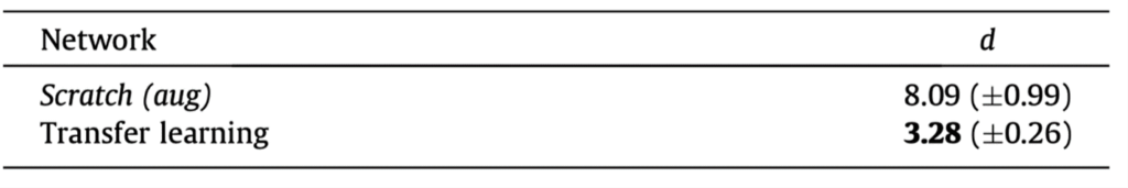
Quantitative metrics for disentanglement in features can be measured using the method proposed by P.P. Brahma et al. (2016). Here, the quantitative metric involves calculating the difference between the Euclidean distance and the geodesic distance between two points in the feature space. In a completely flat manifold, the Euclidean distance and the geodesic distance between the two points are equal. Therefore, smaller values of the quantitative metric proposed by P.P. Brahma et al. (2016) indicate that the features are more disentangled . Calculating the disentanglement quantitative metrics for both networks result in [Table 1]. According to the results, the manifold of features learned by transfer learning is flatter, indicating that it is more disentangled.

Feature disentanglement can also be compared qualitatively. In the early days of deep learning research, the work that established the study of feature disentanglement in deep networks5⁵ defined several characteristics of disentangled features, one of which is that when linear interpolation between features of different classes is performed, the more disentangled the feature, the more plausible the shape ([Figure 8]). In other words, the more disentangled the feature, the flatter the manifold and the more likely it is that the points on the linear interpolation lie on the manifold.

The result of applying these concepts to our research case is shown in [Figure 9]. The middle row visualizes the features of Scratch (aug) and the last row visualizes the features of transfer learning when linearly interpolating between Texture 1 and Texture 2 classes, and between Texture 2 and Texture 5 classes in the DAGM dataset. In the case of Scratch (aug), there are many areas where both classes’ defects coexist during interpolation between different classes. We can see that the features of Scratch (aug) are less disentangled, as explained in [Figure 8]. On the other hand, the features of transfer learning have much fewer overlapping defects during interpolation. This confirms that the features of transfer learning are more disentangled than Scratch (aug).

These quantitative and qualitative experiments confirm that transfer learning’s features are disentangled. Therefore, we can see that transfer learning learns better features in terms of feature disentanglement.

In this article, we’ve explored how to utilize transfer learning in manufacturing and the effect that it can have. SAIGE is currently applying transfer learning to a wide variety of manufacturing data, in addition to the DAGM dataset. We will continue to challenge ourselves to develop specialized technologies for the manufacturing sector.

1. Krizhevsky, A., Sutskever, I. & Hinton, G. E. ImageNet classification with deep convolutional neural networks. Advances in neural information processing systems, 25, 2012, pp.1097-1105. ↩︎
2. Heidelberg Collaboratory for Image Processing, Weakly supervised learning for industrial optical inspection, https://hci.iwr.uni-heidelberg.de/node/3616, 2007, [Online; accessed 19-October-2019]. ↩︎
3. Kim, S., et al. Transfer learning for automated optical inspection. 2017, International Joint Conference on Neural Networks (IJCNN). IEEE. ↩︎
4. Y. Bengio, G. Mesnil, Y. Dauphin, S. Rifai, Better mixing via deep representations, in: Proc. of the 30th International Conference on Machine Learning, Vol. 28, 2013, pp. 552–560.
   Y. Bengio, A. Courville, P. Vincent, Representation learning: a review and new perspectives, IEEE Trans. Pattern Anal. Mach. Intell. 35 (8), 2013, pp.1798–1828. ↩︎
5. Kim, S., Noh. Y.-K., and Park, F. C. Efficient neural network compression via transfer learning for machine vision inspection. Neurocomputing 413, 202, pp.294-304. ↩︎

© SAIGE All Rights Reserved.